PPG Autoencoder Models for Cardiac Anomaly Detection and Signal Quality Screening

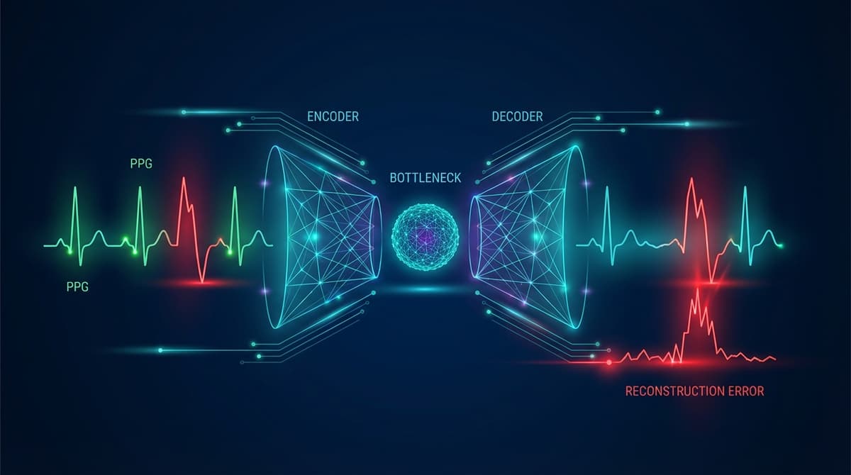
Autoencoders detect cardiac anomalies in PPG signals by learning a compressed representation of normal waveforms during training, then flagging segments where reconstruction error is unusually high at inference time. Because the model only learns what "normal" looks like, any signal that deviates from that learned distribution produces a poor reconstruction, and that reconstruction error becomes the anomaly score. This approach works without labeled abnormal examples, which is a major practical advantage given how rare many cardiac events are in real-world monitoring datasets.

Why Anomaly Detection Matters for Continuous PPG Monitoring

Wearable devices now capture days or weeks of continuous PPG data. The vast majority of that data is ordinary, but the clinically meaningful signal is often buried in a tiny fraction of beats or segments. Traditional rule-based systems set fixed thresholds on heart rate, signal amplitude, or derived features, and they miss patterns that fall outside the designers' expectations. They also generate a lot of false positives from motion artifacts that happen to cross a threshold.

Autoencoders sidestep both problems. They learn the manifold of normal cardiac morphology directly from data, and anything that sits far from that manifold triggers an alert. Arrhythmias, motion artifacts, sensor detachment, and rare cardiac events all have one thing in common from the model's perspective: they look different from normal. The reconstruction error score collapses those diverse failure modes into a single, interpretable number.

This matters for clinical deployment because cardiologists reviewing wearable data do not have time to inspect every beat. An autoencoder-based screening layer can route only the high-reconstruction-error segments to human review, dramatically cutting the annotation burden while improving the chance that rare events are actually caught. Research on long-term Holter recordings has shown that automated anomaly prescreening can reduce review time by more than 70% with minimal sensitivity loss (https://doi.org/10.1016/j.bspc.2021.103027).

Vanilla Autoencoders for PPG Reconstruction

A standard (vanilla) autoencoder consists of an encoder that maps an input segment to a lower-dimensional latent vector, and a decoder that reconstructs the original segment from that vector. The bottleneck forces the network to discard noise and retain only the structure that generalizes across training examples.

For PPG signals, training inputs are typically fixed-length windows of one to five cardiac cycles, normalized to zero mean and unit variance. The encoder might use two or three fully connected layers shrinking from the input dimension down to a bottleneck of 8 to 32 values. The decoder mirrors that structure, expanding back to the original length. Mean squared error between input and reconstruction is the standard training loss.

After training on clean, normal-sinus data, inference is straightforward. Each new window passes through the encoder and decoder, and the MSE between input and output becomes the anomaly score. Segments with scores above a chosen percentile of the training distribution get flagged for review. The threshold can be tuned to balance sensitivity and specificity depending on the clinical context.

One limitation of vanilla autoencoders is that the latent space has no enforced structure. Two normal beats that look similar may map to very different latent vectors, making interpolation unreliable. Variational autoencoders address this.

Variational Autoencoders and PPG Phenotyping

A variational autoencoder (VAE) replaces the deterministic bottleneck with a probabilistic one. The encoder outputs a mean vector and a log-variance vector, and the latent representation is sampled from that Gaussian distribution during training. A KL-divergence term in the loss regularizes the latent space to be approximately standard normal.

The result is a smooth, structured latent space where nearby points correspond to similar waveforms. This has two useful properties for PPG analysis. First, anomalies tend to produce high reconstruction error because unusual waveforms are forced into a latent region that was rarely visited during training, leading to poor decoding. Second, the latent space itself becomes a compact phenotypic fingerprint of cardiac waveform morphology.

Researchers have used VAE latent spaces to cluster PPG recordings from large populations, discovering subgroups that differ in pulse wave velocity, augmentation index, and other hemodynamic markers. The clusters do not always correspond to traditional clinical categories, suggesting that unsupervised phenotyping in latent space may reveal structure that rule-based systems miss. For more on signal preprocessing that feeds these models, see PPG Signal Quality Assessment.

The VAE also supports anomaly scoring through the evidence lower bound (ELBO). A segment that is both hard to reconstruct and has a latent distribution far from the prior will have a low ELBO, providing a more theoretically grounded anomaly score than raw MSE alone.

Convolutional Autoencoders for Temporal Pattern Capture

Fully connected autoencoders treat each time step independently, which loses the local temporal structure of a PPG waveform. Convolutional autoencoders apply convolutional layers in both encoder and decoder, preserving the relative timing of features like the systolic peak, dicrotic notch, and diastolic wave.

A typical architecture stacks three to four convolutional blocks with increasing filter counts and stride-2 downsampling in the encoder, then uses transposed convolutions for upsampling in the decoder. Skip connections borrowed from U-Net architectures can improve reconstruction quality while still allowing the bottleneck to serve as an anomaly discriminator.

Convolutional VAEs combine both ideas: probabilistic latent space with convolutional feature extraction. These models have shown strong performance on tasks like atrial fibrillation detection and premature beat identification, where the shape and timing of the waveform carry diagnostic information that scalar features cannot capture. The connection to supervised arrhythmia classification is explored in detail at PPG Arrhythmia Classification with Machine Learning.

Training on Normal-Only Data: One-Class Classification

The most powerful aspect of autoencoder-based anomaly detection is that it requires only normal examples for training. This is called one-class classification, and it is well-suited to cardiac monitoring for several reasons.

Labeled arrhythmia databases are scarce, expensive to create, and often unrepresentative of the distribution a real deployment will encounter. A model trained on labeled normal-versus-abnormal data will be blind to anomaly types it has never seen. An autoencoder trained only on normal data will, in principle, flag any sufficiently unusual pattern, including novel ones.

Practical one-class training involves three steps. First, collect a large corpus of clean, normal-sinus PPG segments. Signal quality screening (covered in our PPG Signal Quality Assessment guide) is important here: motion artifacts and poor-contact segments should be excluded from training, or the model will learn to reconstruct noise as well as cardiac signal. Second, train the autoencoder to minimize reconstruction error on this corpus. Third, calibrate a threshold on a held-out set of normal segments, setting it at a high percentile (typically 95th to 99th) of the reconstruction error distribution.

At inference time, any segment above the threshold is treated as anomalous. The threshold choice is a clinical parameter. A lower threshold increases sensitivity but also flags more normal-variant waveforms as anomalous. For life-critical applications, a lower threshold with human review is appropriate. For population-scale screening, a higher threshold reduces the review burden.

Detecting Arrhythmias with Reconstruction Error

Atrial fibrillation produces irregular RR intervals and altered waveform morphology. In a well-trained autoencoder, AF segments typically show reconstruction error two to five times higher than sinus rhythm, because the model cannot reconstruct the irregular inter-beat spacing or the dampened waveform shape that accompanies AF. Published benchmarks on the PhysioNet AF challenge dataset have reported AUROC values above 0.90 for VAE-based detectors trained without any AF examples (https://doi.org/10.1088/1361-6579/ac3b5b).

Premature atrial and ventricular contractions show a brief morphological deviation followed by a compensatory pause. The autoencoder reconstruction error spikes on the ectopic beat and often on the post-ectopic beat as well. This double-spike pattern can help differentiate isolated ectopy from sustained arrhythmia.

Second- and third-degree heart block produce dramatically slowed heart rate with normal individual beat morphology. A segment-level autoencoder may miss these if trained on variable-rate normal data. Beat-level autoencoders, which reconstruct individual waveforms rather than multi-beat segments, are more sensitive to morphological anomalies, while segment-level models are more sensitive to rhythm anomalies.

Motion Artifact Identification and Signal Quality Screening

Motion artifacts are a persistent challenge in wearable PPG. They corrupt the signal with high-frequency noise and low-frequency baseline wander, making downstream heart rate and SpO2 estimates unreliable. Standard approaches use accelerometer data to detect motion periods, but accelerometer-free quality screening is useful when the sensor does not include a motion sensor.

An autoencoder trained on clean, stationary-period PPG will produce high reconstruction error on motion-corrupted segments because the artifact morphology differs substantially from the training distribution. This provides a purely optical quality score that correlates well with accelerometer-based motion labels, even though no accelerometer data was used. The PPG Signal Quality Assessment article covers how these scores integrate into a broader quality pipeline.

Sensor detachment, pressure artifacts from tight straps, and optical interference from ambient light all produce distinctive artifact patterns. Because the autoencoder flags anything unusual, it catches all of these failure modes under a single scoring function rather than requiring separate detectors for each artifact type.

Comparison with Threshold-Based Anomaly Detection

Traditional threshold-based systems monitor scalar features: heart rate, pulse amplitude, signal-to-noise ratio. When any feature crosses a preset limit, an alert fires. These systems are transparent and easy to audit, but they have several weaknesses.

They require domain experts to decide which features matter and where the thresholds should sit. They are brittle to population heterogeneity: a threshold calibrated on young healthy adults may be inappropriate for elderly patients with naturally lower pulse amplitudes. And they cannot detect anomalies that manifest in waveform shape rather than scalar summary statistics.

Autoencoders capture the full waveform distribution, not just a handful of hand-crafted features. They adapt to individual baselines if fine-tuned on each user's personal normal data. And because reconstruction error is a continuous score, the alert threshold can be adjusted after deployment without retraining the model.

The tradeoff is interpretability. When a threshold-based system fires an alert, the reason is explicit. When an autoencoder fires an alert, the high reconstruction error tells you that something is unusual but not precisely what. Post-hoc attribution methods like saliency maps and integrated gradients can highlight which parts of the waveform contributed most to the error, partially recovering interpretability. For a broader look at how these models fit into production systems, see the PPG Machine Learning Pipeline guide.

Practical Considerations for Deployment

Several engineering choices affect real-world autoencoder performance. Model size matters for edge deployment on wearables with limited compute budgets. Quantized convolutional autoencoders can run on microcontrollers with under 100KB of RAM, enabling on-device anomaly scoring rather than cloud offload.

Training data diversity is equally important. A model trained on data from one sensor type or one demographic group may underperform on others. Data augmentation techniques such as time stretching, amplitude scaling, and additive noise can improve generalization. The PPG Data Augmentation article covers these strategies in detail.

Continual learning is an open research problem. A model deployed for months will encounter distribution shifts as the user ages, gains or loses weight, or develops new conditions. Periodic re-calibration of the anomaly threshold, or light fine-tuning on recent personal data, can maintain performance over time.

Frequently Asked Questions

What is reconstruction error in a PPG autoencoder?

Reconstruction error is the difference between the original PPG segment fed into the autoencoder and the segment that the decoder produces from the compressed latent representation. It is usually measured as mean squared error or mean absolute error over the time steps in the window. High reconstruction error means the model struggled to reproduce the input, which indicates the segment is unlike the normal training data.

Can an autoencoder detect atrial fibrillation in PPG without labeled AF data?

Yes. A VAE or convolutional autoencoder trained only on normal sinus rhythm will typically produce substantially higher reconstruction error on AF segments because AF alters both the inter-beat rhythm and the waveform shape. Published studies using PhysioNet data report AUROC values above 0.90 for this approach. However, performance varies depending on training data quality and the specific AF patterns present.

How does a variational autoencoder differ from a standard autoencoder for PPG anomaly detection?

A standard autoencoder maps each input to a single point in latent space. A variational autoencoder maps each input to a probability distribution, and the latent space is regularized to follow an approximately standard normal distribution. This makes the latent space smoother and more structured, which improves anomaly scoring (using the ELBO rather than raw MSE) and enables phenotyping of waveform subgroups through latent space clustering.

How much data is needed to train a PPG autoencoder?

A rough guideline is tens of thousands of clean, labeled-normal beat or segment windows. The exact number depends on the complexity of the architecture and the diversity of the training population. More diverse data generally improves generalization. Models trained on publicly available databases like MIMIC-III or the PhysioNet waveform databases can serve as starting points for fine-tuning on specific deployment populations.

Can autoencoders replace signal quality indices for PPG?

Autoencoders can serve as a flexible, learned signal quality score that captures artifact types no hand-crafted index was designed for. They work best as a complement to, rather than replacement for, established signal quality indices. Combining the reconstruction error score with physiological plausibility checks (heart rate in a reasonable range, waveform amplitude above sensor noise floor) produces more robust quality filtering than either approach alone.

What are the main failure modes of PPG autoencoder anomaly detection?

The main failure modes are: training data contamination (if the training set includes undetected artifacts or arrhythmias, the model learns to reconstruct them without error); distribution shift (a model trained on one population or sensor may not generalize to others); and false positives from normal physiological variation (deep breathing, exercise, or positional changes can temporarily alter PPG morphology enough to trigger elevated reconstruction error without any pathology present).

How do I choose the anomaly threshold for a deployed autoencoder?

The threshold is typically set at a high percentile of reconstruction errors observed on a held-out set of known-normal segments: the 95th or 99th percentile are common starting points. In clinical applications, the threshold should be validated against labeled abnormal examples from the target population before deployment. For consumer wellness applications, a higher threshold with lower alert rate is usually preferred to avoid alarm fatigue.